의사결정나무(DecisionTree)
- 데이터를 분류할때 특정 기준에 따라 "예" / "아니오"로 답할 수 있는 질문을 이어 나가면서 학습
- 원본데이터에서 계속 규칙을 만들면서 가지치기 함
- 따라서 결정트리를 이용한 예측결과는 분류 규칙이 명확해서 해석이 쉬움
- 독립변수와 종속변수에 연속형, 명목형 변수를 모두 사용 가능
- 선형성, 정규성 등의 가정이 필요하지 않음
| 구분 | 내용 |
| 장점 | - 모델을 쉽게 설명할 수 있고 시각화 하기 편함 - 이상치, 전처리 등에 모델의 성능이 크게 영향을 받지 않음 - 정규화나 표준화 등의 전처리를 요구하지 않음 |
| 단점 | - 복잡도를 제어하더라도 과대적합의 가능성이 높아 일반화 성능이 우수하지 않음(이를 해결하기 위해 앙상블 기법 제안) |
[생성]
- 학습의 의미: 정답에 가장 빨리 도달하는 질문목록 학습
- 데이터를 통해 최적의 분리규칙을 찾아 질문목록을 생성
- 트리를 성장시키는 과정에서 적절한 정지규칙을 만족하면 트리의 자식마디 생성을 중단
- 분리기준 설정
| 종속변수 형태 | 지도학습 문제 | 분리기준 | 내용 | ||
| 이산형 | 분류 | 카이제곱 p-value | p-value가 가장 작은 예측 변수와 그 때의 최적분리에 의해 자식마디 형성 | ||
| 지니지수 | 지니지수가 최소가 되는 방향으로 분리 | ||||
| 엔트로피 | 엔트로피지수가 최소가 되는 방향으로 분리 | ||||
| 연속형 | 회귀 | F통계량 | p-value가 가장 작은 쪽으로 분리 | ||
| 분산감소량 | 분산의 감소량이 최대가 되는 방향으로 분리 | ||||
[복잡도 제어]
- 복잡도: 트리의 크기
- 모든 데이터가 분할되도록 하는 모델을 생성하면 해당데이터에 높은 예측을 갖음
- 하지만 과대적합되어 다른 데이터에서는 예측력이 떨어질 수 있음
- 이를 방지하기 위해 가지지치기(pruning)를 이용
- sklearn에서는 사전가지치기(Pre-pruning)를 사용
- 사전가지치기 종류에는 트리의 최대 깊이 제한, 리프의 최대 개수 제한, 노드 분할을 위한 포인트의 최소 개수 지정
[변수중요도]
- 트리가 어떻게 작동했는지 속성을 살펴볼 수 있음
- 변수중요도: 트리를 만드는 결정에 변수가 어떻게 작용했는지 확인(0~1사이값을 갖음)
- 변수중요도가 0일 경우 트리를 만드는 과정에 해당 변수가 전혀 작용하지 않음
- 변수중요도가 1일 경우 트리를 만드는 과정에 목푯값을 완전하게 예측
- 변수중요도의 총 합은 1
- 변수중요도 값은 항상 양수
- 목표값에 대해 어떤 클래스를 지지하는지 알 수 없음
[모델]
sklearn.tree.DecisionTreeClassifier(parameters)
sklearn.tree.DecisionTreeClassifier
Examples using sklearn.tree.DecisionTreeClassifier: Release Highlights for scikit-learn 1.3 Classifier comparison Plot the decision surface of decision trees trained on the iris dataset Post prunin...
scikit-learn.org
예시) 독일 신용데이터를 활용해 결정트리 분류분석 수행
- 데이터정의
- 데이터분리
- 종속변수: credic.rating
- 독립변수: 나머지
- 원데이터에서 종속변수는 0과 1로 나누어져 있고 3:7의 비율임
- 학습용데이터와 테스트용 데이터를 분리할때도 원데이터의 비율과 동일하게 하기 위해 stratify=y를 적용
#데이터 분리
X = credit.drop(columns=["credit.rating"], axis=1)
y = credit["credit.rating"]
print(X.shape)
print(y.shape)

y.value_counts()

from sklearn.model_selection import train_test_split

x_train, x_test, y_train, y_test = train_test_split(X, y, test_size=.3, stratify=y, random_state=0)

print(x_train.shape, y_train.shape)
print(x_test.shape, y_test.shape)

'''
(700, 20) (700,)
(300, 20) (300,)
'''
- 학습, 예측, 평가
- 정확도 70%로 나타남
#학습
from sklearn.tree import DecisionTreeClassifier

clf = DecisionTreeClassifier(max_depth=5)

clf.fit(x_train, y_train)

#예측 및 평가
from sklearn.metrics import confusion_matrix, classification_report

pred = clf.predict(x_test)

cm = confusion_matrix(y_test, pred)
'''
array([[ 34,  56],
       [ 35, 175]])
'''

cr = classification_report(y_test, pred)
'''
 		precision    recall  f1-score   support

           0       0.49      0.38      0.43        90
           1       0.76      0.83      0.79       210

    accuracy                           0.70       300
   macro avg       0.63      0.61      0.61       300
weighted avg       0.68      0.70      0.68       300

'''
- roc_curve확인
#roc curve확인
from sklearn.metrics import roc_auc_score, RocCurveDisplay

roc_score = roc_auc_score(y_test, clf.predict_proba(x_test)[:,1])
print(f"roc_auc_score: {roc_score}")
RocCurveDisplay.from_estimator(clf, x_test, y_test)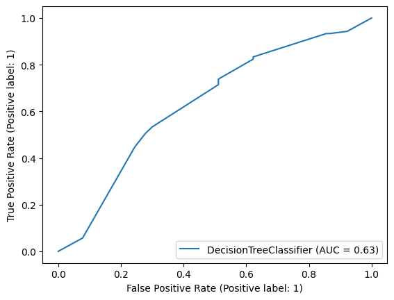
- 변수중요도 확인
#변수중요도 확인
importance = clf.feature_importances_

importance_cols = X.columns
importance_df = pd.DataFrame({
    "feature_name": importance_cols,
    "importance": importance
})
importance_df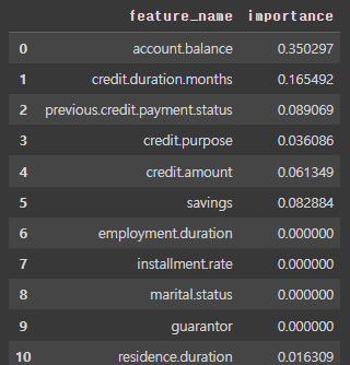
- 의사결정나무 확인
#의사결정나무 그리기
import pydot
import pydotplus
import graphviz
from sklearn.tree import export_graphviz

dt_dot_data = export_graphviz(
    clf,
    feature_names=X.columns,
    class_names=np.array(["0", "1"]),
)

dt_graph = pydotplus.graph_from_dot_data(dt_dot_data)

from IPython.display import Image

Image(dt_graph.create_png())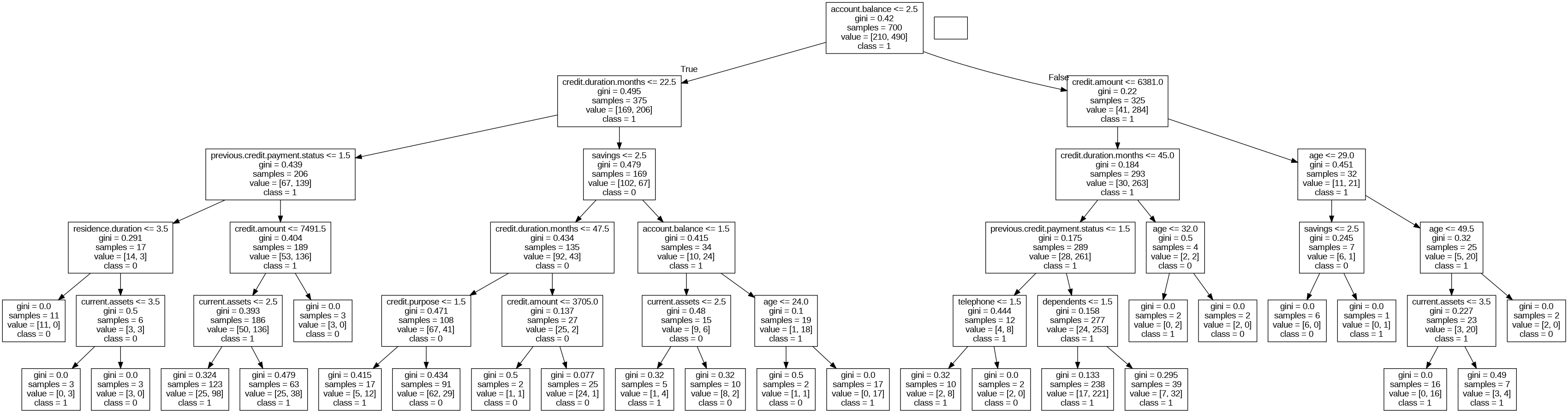
sklearn.tree.DecisionTreeRegressor(parameters)
sklearn.tree.DecisionTreeRegressor
Examples using sklearn.tree.DecisionTreeRegressor: Release Highlights for scikit-learn 0.24 Release Highlights for scikit-learn 0.22 Decision Tree Regression Multi-output Decision Tree Regression D...
scikit-learn.org
예시) 임의 데이터로 의사결정나무 회귀 수행
- 데이터정의
#임의 데이터 생성
X = np.sort(5 * np.random.rand(400, 1), axis=0)
y = np.sin(X).ravel()
T = np.linspace(0, 5, 500)[:,np.newaxis]
- 데이터분할
#데이터분할
x_train, x_test, y_train, y_test = train_test_split(X, y, test_size=.3, random_state=1)
print(x_train.shape, y_train.shape)
print(x_test.shape, y_test.shape)
- 학습, 예측, 평가
#모델생성
from sklearn.tree import DecisionTreeRegressor

dcr1 = DecisionTreeRegressor(max_depth=2)
dcr2 = DecisionTreeRegressor(max_depth=5)

pred1 = dcr1.fit(x_train, y_train).predict(x_test)
pred2 = dcr2.fit(x_train, y_train).predict(x_test)

#예측 및 평가
from sklearn.metrics import mean_absolute_error, mean_squared_error

indexes = ["max_depth=2", "max_depth=5"]
columns = ["mae", "mse", "rmse"]
preds = [pred1, pred2]

results = pd.DataFrame(
    index=indexes, columns=columns
)

for pred, index in zip(preds, indexes):
  mae = mean_absolute_error(y_test, pred)
  mse = mean_squared_error(y_test, pred)
  rmse = mean_squared_error(y_test, pred, squared=False)

  results.loc[index, "mae"] = mae
  results.loc[index, "mse"] = mse
  results.loc[index, "rmse"] = rmse

results

'''
		mae		mse		rmse
max_depth=2	0.165072	0.045096	0.212357
max_depth=5	0.034897	0.002249	0.047419
'''
- 시각화
- 트리의 깊이가 깊어짐에 따라 예측선이 원데이터에 더 디테일하게 맞춰지는 것을 볼 수 있다.
dcrs = [dcr1, dcr2]
depths = ["max_depth=2", "max_depth=5"]
plt.figure(figsize=(15, 5))
for i, dcr in enumerate(dcrs):
  pred = dcr.fit(X, y).predict(T[:400])
  r2 = dcr.score(T[:400], pred)
  mae = mean_absolute_error(y, pred)

  plt.subplot(1, 2, i+1)
  plt.scatter(X, y, s=20, c="darkorange", label="data")
  plt.plot(T[:400], pred, c="navy", label=depths[i])
  plt.title(f"R2: {r2}, mae: {mae:.2f}")
  plt.xlabel("data")
  plt.ylabel("pred", rotation=90)
  plt.legend()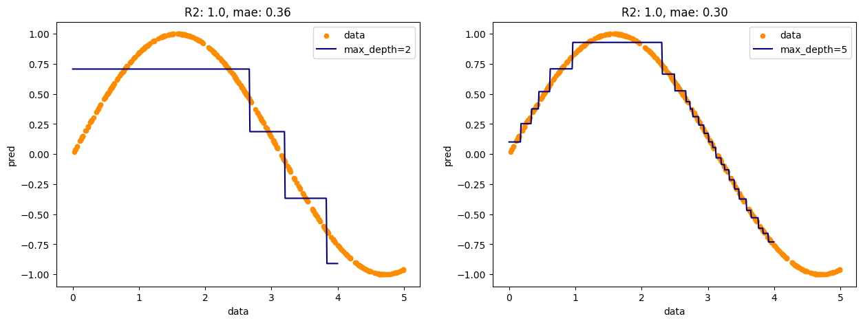
'Data Analysis > Machine Learning' 카테고리의 다른 글
| Python_ML_Supervised_KNN (1) | 2024.02.28 |
|---|---|
| Python_ML_Supervised_SVM (0) | 2024.01.03 |
| Python_ML_Supervised_Multiple Regression (0) | 2024.01.02 |
| Python_ML_Supervised_Polynomial Regression (0) | 2024.01.02 |
| Python_ML_Supervised_SimpleLinearRegression (0) | 2024.01.02 |


