Data Analysis/Machine Learning
Python_ML_Supervised_SVM
mansoorrr
2024. 1. 3. 15:17
서포트벡터머신(SVM: Support Vector Machine)
- 새로운 데이터가 입력되었을때, 기존데이터를 활용해 분류하는 방법
- SVM은 최대마진분류기(Maximal Margin Classifier)를 일반화 한 것
- 최대마진분류기의 단점을 보완한 것이 SVC(Support Vector Classifier)
- SVC를 더 확장하고 비선형 클래스 경계를 수용하기 위해 SVM고안
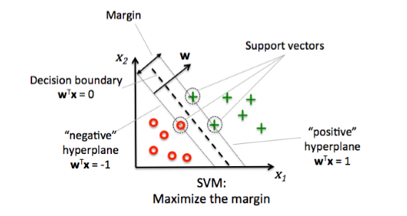
[최대마진분류기]
- 초평면(Hyperplane)
- p차원인 공간에서 (p-1)차원인 평평한 부분공간
- ex) 2차원일 경우 초평면은 1차원인 선이 되고, 3차원일 경우 초평면은 2차원인 면이 됨
- 데이터를 두 공간으로 나눌 수 있는 초평면은 무한개
- 무한개의 초평면 중 어느것을 최종으로 사용할지 결정해야 함
- p차원인 공간에서 (p-1)차원인 평평한 부분공간
- 마진(Margin)
- 데이터에서 초평면까지의 거리
- 마진이 가장 큰 초평면을 찾음
- 서포트벡터(Support Vector)
- 양의 초평면과 음의 초평면에 접한 관측값들
- 초평면으로 데이터 클래스를 분류하면 학습데이터를 완벽하게 분류하기 때문에 과적합의 위험과 이상치에 민감하다는 특징이 있음
[SVC]
- 모든 데이터가 초평면에 의해 두 영역으로 분리될 수 있는 것이 아님
- 따라서 이상치로부터 영향을 덜 받으면서 대부분의 학습데이터를 잘 분류할 수 있는 방식을 고안
- 최대마진분류기를 가지면서도 일부 관측치들이 마진이나 초평면의 반대쪽에 있는 것을 허용
- 데이터 클래스가 두 영역으로 나뉘고 그 사이의 경계가 선형인 경우 사용 가능
- sklearn.svm.SVC(parameters)
| Parameter | |
| C | - default=1.0 - 정규화파라미터로 정규화 강도는 C에 반비례 - 반드시 양수여야 하며 |
| kernel | - default: rbf - 커널함수의 타입 선택 - linear, poly, rbf, sigmoid, precomputed중 선택 |
| degree | - default: 3 - 커널함수를 poly로 선택했을 때 다항함수의 차수 |
| gamma | - default: scale - 커널함수가 rbf, poly, sigmoid일때 커널의 계수를 의미 - scale: 1/(n_features*X.var()) - auto: 1/n_features |
| coef() | - default: 0.0 - 커널함수를 poly, sigmoid로 선택했을때, 커널 함수의 독립항을 지정 |
| tol | - default: 1e-3 - 중지기준 |
| class_weight | - default: None - default일 경우 모든 클래스에 대해 가중치를 1로 적용 - 각 클래스에서 매개변수 C에 대해 class_weight[i]*C로 가중치를 부여 |
| verbose | - default: 0 - 자세한 진행 수준 |
| max_iter | - default: 1000 - 최대 실행 반복 횟수 |
| decision_function_shape | - default: ovr - ovo: one vs one 방식 - ovr: one vs rest 방식 |
| probability | - default: False - 클래스에 할당되는 확률 추정 여 |
| Property | |
| class_weight_ | - 각 클래스에 대한 파라미터 C의 승수 |
| coef_ | - kernel="linear" 일때 변수에 할당된 가중치 |
| duel_coef_ | - 결정 함수에서 서포트 벡터에 대한 이중 계수 |
| intercept_ | - decision_function의 상수 |
| support_vercotrs_ | - 서포트벡터들 |
| support_ | - 서포트벡터의 인덱스 |
| n_support_ | - 각 클래스에 대한 서포트 벡터의 개수 |
| Method | |
| decision_function(X) | - 데이터 샘플의 Confidence Score |
| fit(X, y) | - 모델 학습 |
| get_params([deep]) | - 모델의 매개변수 가져오기 |
| predict(X) | - 예측값 |
| predict_proba(X) | - 클래스에 대한 예측 확률 |
| predict_log_proba(X) | - 클래스에 대한 예측 로그 확률 |
| score(X, y) | - 예측의 평균 정확 |
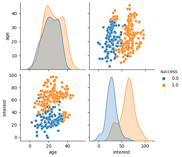
예시1) kaggle의 classification데이터로 svc진행
- 데이터 로드 및 분포 파악
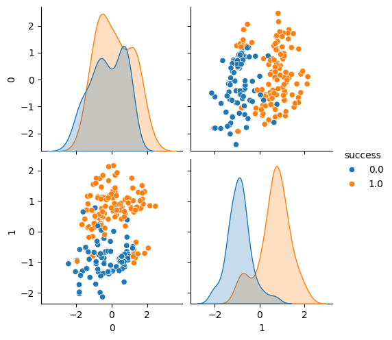
- SVC는 스케일에 민감해서 StandardScaling을 적용하면 구분이 더 뚜렷하게 나타남
#---------- data로드
print(data.shape)
data.head()

#데이터 분포 파악
sns.pairplot(data=data, hue="success")

#스케일링 후 분포 파악
from sklearn.preprocessing import StandardScaler

scaler = StandardScaler()
scaled_x_train = scaler.fit_transform(x_train)

sns.pairplot(data=pd.concat(
    [pd.DataFrame(scaled_x_train), y_train.reset_index(drop=True)],
    axis=1
), hue="success")
- 모델적용(1): 기본데이터
- 데이터 분리
from sklearn.model_selection import train_test_split

X = data.drop(["success"], axis=1)
y = data["success"]

x_train, x_test, y_train, y_test = train_test_split(X, y, test_size=.3, random_state=1)

print(x_train.shape, y_train.shape) #(207, 2) (207,)
print(x_test.shape, y_test.shape) #(90, 2) (90,)
- 모델학습 및 평가
- proba=0.5를 기준으로 클래스를 예측하는것이 달라짐
- confidence score가 양수이면 class1일 확률이 높아지고 음수이면 class0일 확률이 높아짐
from sklearn.svm import SVC

svc = SVC(probability=True) # proba를 구하기 위해 probability=True로 설정
svc.fit(x_train, y_train)

proba = svc.predict_proba(x_train) #proba산출
cs = svc.decision_function(x_train) #confidence score 산출

cs_df = pd.DataFrame(cs, columns=["cs"])
cs_df[["class0", "class1"]] = proba

#confidence score에 따른 class별 proba 확인
plt.plot(cs_df["cs"], cs_df["class0"], "g*", label="class0")
plt.plot(cs_df["cs"], cs_df["class1"], "r.", label="class1")
plt.xlabel("confidence score")
plt.ylabel("proba")
plt.legend()
plt.show();

- C(정규화 강도)에 따른 score차이확인
- C의 크기와 정규화 강도는 반비례
- C의 크기가 커짐에 따라 score가 올라감(과적합 가능성 있을 수 있음)
c_list = np.arange(0.1, 3.1, 0.1)
# c_list = [0.1, 0.3, 0.5, 0.7, 1.0, 1.3, 1.5, 1.7, 2.0]
scores = []
probs =[]
for c in c_list:
  svc = SVC(C=c, probability=True)
  svc.fit(x_train, y_train)
  scores.append(svc.score(x_train, y_train))
  probs.append(svc.predict_proba(x_train))

 plt.plot(c_list, scores)
 plt.xlabel("C")
 plt.ylabel("score")
 plt.show();
- 정확도 및 분류 기준표 확인
svc.score(x_train, y_train) #0.9082125603864735

pred = svc.predict(x_test) #예측

from sklearn.metrics import confusion_matrix, accuracy_score, precision_score, recall_score, f1_score

cfm = confusion_matrix(y_test, pred)
acc = accuracy_score(y_test, pred)
prc = precision_score(y_test, pred)
recall = recall_score(y_test, pred)
f1 = f1_score(y_test, pred)

print(f"[confusion matrix]\n{cfm}")
print(f"accuracy: {acc}")
print(f"precision: {prc}")
print(f"recall: {recall}")
print(f"f1: {f1}")

'''
[confusion matrix]
[[39  2]
 [ 8 41]]
accuracy: 0.8888888888888888
precision: 0.9534883720930233
recall: 0.8367346938775511
f1: 0.8913043478260869
'''- 모델적용(2): 스케일링 적용
- 데이터 정의
- 테스트데이터에 스케일링 적용
scaled_x_test = scaler.transform(x_test)- 학습 및 예측
- 기본 데이터로 진행했을때 보다 스케일링 진행 후 모델의 성능이 올라갔음을 알 수 있다.
#모델정의
scaled_svc = SVC()
scaled_svc.fit(scaled_x_train, y_train)
scaled_svc.score(scaled_x_train, y_train) #0.9227053140096618

scaled_pred = scaled_svc.predict(scaled_x_test)
scaled_cfm = confusion_matrix(y_test, scaled_pred)
scaled_acc = accuracy_score(y_test, scaled_pred)
scaled_prc = precision_score(y_test, scaled_pred)
scaled_recall = recall_score(y_test, scaled_pred)
scaled_f1 = f1_score(y_test, scaled_pred)

print(f"[confusion matrix]\n{scaled_cfm}")
print(f"accuracy: {scaled_acc}")
print(f"precision: {scaled_prc}")
print(f"recall: {scaled_recall}")
print(f"f1: {scaled_f1}")

'''
[confusion matrix]
[[41  0]
 [ 4 45]]
accuracy: 0.9555555555555556
precision: 1.0
recall: 0.9183673469387755
f1: 0.9574468085106383
'''
[SVM]
- 데이터의 형태가 비선형일 경우 커널(Kernel)을 활용해 SVC개념을 확장
- Kernel: 두 관측치들의 유사성을 수량화 하는 함수
- ex) 2차원의 비선형 데이터를 3차원으로 변환하면 선형 분리가 가능
[SVR]
- SVM개념을 활용해 회귀분석 실시
- 분류기에서는 마진을 최대화 하는 길을 구했지만 회귀에서는 마진안에 가능한 많은 데이터가 들어가게 학습
- 도로 밖의 데이터샘플을 마진 오류라고 함
- 가장 많이 사용하는 손실함수는 epsilon-insensitive

| Parameter | |
| C | - default=1.0 - 정규화파라미터로 정규화 강도는 C에 반비례 - 반드시 양수 |
| kernel | - default: rbf - 커널함수의 타입 선택 - linear, poly, rbf, sigmoid, precomputed중 선택 |
| degree | - default: 3 - 커널함수를 poly로 선택했을 때 다항함수의 차수 |
| gamma | - default: scale - 커널함수가 rbf, poly, sigmoid일때 커널의 계수를 의미 - scale: 1/(n_features*X.var()) - auto: 1/n_features |
| coef() | - default: 0.0 - 커널함수를 poly, sigmoid로 선택했을때, 커널 함수의 독립항을 지정 |
| tol | - default: 1e-3 - 중지기준 |
| verbose | - default: 0 - 자세한 진행 수준 |
| max_iter | - default: 1000 - 최대 실행 반복 횟수 |
| Property | |
| class_weight_ | - 각 클래스에 대한 파라미터 C의 승수 |
| coef_ | - kernel="linear" 일때 변수에 할당된 가중치 |
| duel_coef_ | - 결정 함수에서 서포트 벡터에 대한 이중 계수 |
| intercept_ | - decision_function의 상수 |
| support_vercotrs_ | - 서포트벡터들 |
| support_ | - 서포트벡터의 인덱스 |
| n_support_ | - 각 클래스에 대한 서포트 벡터의 개수 |
예시1) 임의의 데이터로 SVR진행
- 데이터생성
X = np.sort(np.random.rand(40, 1), axis=0)
y = np.sin(X).ravel()

#y에 노이즈 추가
y[::5] += 3*(0.5-np.random.rand(8))
- 모델 학습 및 평가
- kernel을 "rbf", "linear", "poly" 세개로 변경하며 모델 적합도 확인
from sklearn.svm import SVR

svr_rbf = SVR(kernel="rbf", gamma=0.1, C=100, epsilon=0.1)
svr_linear = SVR(kernel="linear", gamma="auto", C=100)
svr_poly = SVR(kernel="poly", degree=3, gamma="auto", C=100, epsilon=0.1, coef0=1)

#학습
svr_rbf.fit(X, y)
svr_linear.fit(X, y)
svr_poly.fit(X, y)

rbf_pred = svr_rbf.predict(X)
linear_pred = svr_linear.predict(X)
poly_pred = svr_poly.predict(X)

kernels = ["rbf", "linear", "poly"]
evals = ["mae", "mse", "rmse"]

preds = [rbf_pred, linear_pred, poly_pred]

results = pd.DataFrame(index=kernels, columns=evals)

from sklearn.metrics import mean_squared_error, mean_absolute_error

#평가
for pred, kernel in zip(preds, kernels):
  mae = mean_absolute_error(y, pred)
  mse = mean_squared_error(y, pred)
  rmse = mean_squared_error(y, pred, squared=False)

  results.loc[kernel, "mae"] = mae
  results.loc[kernel, "mse"] = mse
  results.loc[kernel, "rmse"] = rmse

results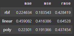
- 시각화
#시각화
svrs = [svr_rbf, svr_linear, svr_poly]
kernels = ["RBF", "Linear", "Polynomial"]
svrs_colors = ["m", "c", "g"]

fig, axes = plt.subplots(nrows=1, ncols=3, figsize=(15, 7), sharey=True)

for i, svr in enumerate(svrs):
  axes[i].plot(
      X,
      svr_rbf.fit(X, y).predict(X),
      color=svrs_colors[i],
      lw=2,
      label=f"{kernels[i]} model"
  )
  axes[i].scatter(
      X[svr.support_],
      y[svr.support_],
      edgecolor=svrs_colors[i],
      s=50,
      label=f"{kernels[i]} support vectors"
  )
  axes[i].scatter(
      X[np.setdiff1d(np.arange(len(X)), svr.support_)],
      y[np.setdiff1d(np.arange(len(X)), svr.support_)],
      edgecolor=svrs_colors[i],
      s=50,
      label=f"other training data"

  )
  axes[i].legend(
      loc="upper center",
      bbox_to_anchor=(0.5, 1.1),
      ncol=1
  )

plt.show();